The Sinc Function

In the 4th edition of Intermediate Physics for Medicine and Biology, Russ Hobbie and I discuss many mathematical functions, from common ones like the sine function and the exponential function to less familiar ones like Bessel functions and the error function. A simple but important example is the sinc function.

Sinc(x) is defined as sin(x)/x. It is zero wherever sin(x) is zero (where x is a multiple of π), except at x = 0, where sinc is one. The shape of the sinc function is a central peak surrounded by oscillations with decaying amplitude.

The sinc function.

The most important property of the sinc function is that it is the Fourier transform of a square pulse. In Chapter 18 about magnetic resonance imaging, a slice of a sample is selected by turning on a magnetic field gradient, so the Larmor frequencies of the hydrogen atoms depend on location. To select a uniform slice, you need to excite hydrogen atoms with a uniform range of Larmor frequencies. The radio-frequency pulse you must apply is specified by its Fourier transform. It is an oscillation at the central Larmor frequency, with an amplitude modulated by a sinc function.

When you integrate sinc(x), you get a new special function that Russ and I never discuss: the sine integral function, Si(x)

The sine integral function, Si(x).

This function looks like a step function, but with oscillations. As x goes to infinity the sine integral approaches π/2. It is odd, so as x goes to minus infinity it approaches –π/2.

The sinc function and the sine integral function resemble the Dirac delta function and the Heaviside step function. In fact, sinc(x/a)/a gets taller and taller, and the side lobes fall off faster and faster, as a approaches zero; it becomes the delta function.Similarly, the sine integral function becomes—to within a constant term, π/2—the step function.

Special functions often have interesting and beautiful properties. As I noted earlier, if you integrate sinc(x) from zero to infinity you get π/2. However, if you integrate the square of sinc(x) from zero to infinity you get the same result: π/2. These two functions are different: sinc(x) oscillates between negative and positive values, so its integral oscillates from above π/2 to below π/2, as shown above; sinc²(x) is always positive, so its integral grows monotonically to its asymptotic value. But as you extend the integral to infinity, the area under these two curves is exactly the same! I’m not sure there is any physical significance to this property, but it is certainly a fun fact to know.

Electron Paramagnetic Resonance Imaging

Magnetic resonance comes in two types: nuclear magnetic resonance and electron paramagnetic resonance. In Chapter 18 of the 4th edition of Intermediate Physics for Medicine and Biology, Russ Hobbie and I write

Two kinds of spin measurements have biological importance. One is associated with electron magnetic moments and the other with the magnetic moments of nuclei. Most neutral atoms in their ground state have no magnetic moment due to the electrons. Exceptions are the transition elements that exhibit paramagnetism. Free radicals, which are often of biological interest, have an unpaired electron and therefore have a magnetic moment. In most cases this magnetic moment is due almost entirely to the spin of the unpaired electron.

Magnetic resonance imaging is based on the magnetic moments of atomic nuclei in the patient. The total angular momentum and magnetic moment of an atomic nucleus are due to the spins of the protons and neutrons, as well as any orbital angular momentum they have inside the nucleus. Table 18.1 lists the spin and gyromagnetic ratio of the electron and some nuclei of biological interest.

The key insight from Table 18.1 is that the Larmor frequency for an electron in a magnetic field is about a thousand times higher than for a proton. Therefore, MRI works at radio frequencies, whereas EPR imaging is at microwave frequencies. Can electron paramagnetic resonance be used to make images like nuclear magnetic resonance can? I should know the answer to this question, because I hold two patents about a “Pulsed Low Frequency EPR Spectrometer and Imager” (U.S. Patents 5,387,867 and 5,502,386)!

I’m not particularly humble, so when I tell you that I didn’t contribute much to developing the EPR imaging technique described in these patents, you should believe me. The lead scientist on the project, carried out at the National Institutes of Health in the mid 1990s, was John Bourg. John was focused intensely on developing an EPR imager. Just as with magnetic resonance imaging, his proposed device needed strong magnetic field gradients to map spatial position to precession frequency. My job was to design and build the coils to produce these gradients. The gradients would need to be strong, so the coils would get hot and would have to be water cooled. I worked on this with my former boss Seth Goldstein, who was a mechanical engineer and therefore know what he was doing in this design project. Suffice to say, the coils never were built, and from my point of view all that came out of the project was those two patents (which have never yielded a dime of royalties, at least that I know of). This project was probably the closest I ever have come to doing true mechanical engineering, even though I was a member of the Mechanical Engineering Section when I worked in the Biomedical Engineering and Instrumentation Program at NIH.

One of our collaborators, Sankaran Subramanian, continued to work on this project for years after I left NIH. In a paper in Magnetic Resonance Insights, Subramanian describes his work in “Dancing With The Electrons: Time-Domain and CW In Vivo EPR Imaging” (Volume 2, Pages 43–74, 2011). Below is an excerpt from the introduction of his article, with references removed. It provides an overview of the advantages and disadvantages of EPR imaging compared to MRI.

Magnetic resonance spectroscopy, in general, deals with the precessional frequency of magnetic nuclei, such as ¹H, ¹³C, ¹⁹F, ³¹P, etc. and that of unpaired electrons in free radicals and systems with one or more unpaired electrons when placed in a uniform magnetic field. The phenomena of nuclear induction and electron resonance were discovered more or less at the same time, and have become two of the most widely practiced spectroscopic techniques. The finite dimensional spin space of magnetic nuclei makes it possible to quantum mechanically precisely predict how the nuclear spin systems will behave in a magnetic field in presence of radiofrequency fields. On the other hand, the complex and rather diffuse wave functions of the unpaired electron which get further influenced by the magnetic vector potential make it a real challenge to predict the precise behavior of electron resonance systems. The subtle variations in the precessional frequencies brought about by changes in the electronic environment of the magnetic nuclei in NMR and that of the unpaired electrons in EPR make the two techniques widely practiced and very useful in the structural elucidation of complex biomolecules. It was discovered subsequently that the presence of linear field gradients enabled precise spatial registration of nuclear spins which led to the development of imaging of the distribution of magnetic nuclei establishing an important non-invasive medical imaging modality of water-rich soft tissues in living systems with its naturally abundant presence of protons. Nuclear Magnetic Resonance Imaging, popularly known as MRI, is now a well-known and indispensable tool in diagnostic radiology. …

The entirely analogous field of electron paramagnetic (spin) resonance (EPR or ESR) that deals with unpaired electron systems developed as a structural tool much more rapidly with the intricate spectra of free radicals and metal complexes providing an abundance of precise structural information on molecules, that would otherwise be impossible to unravel. The spectroscopic practice of EPR traditionally started in the microwave region of the electromagnetic spectrum and was essentially a physicist’s tool to study magnetic properties and the structure of paramagnetic solid state materials, crystal defects (color centers), etc. Later, chemists started using EPR to unravel the structure of organic free radicals and paramagnetic transition metal and lanthanide complexes. Early EPR instrumentation closely followed the development of radar systems during the Second World War and was operating in the X-band region of the electromagnetic spectrum (~9 GHz). Pulsed EPR methods developed somewhat later due to the requirement of ultra fast switches and electronic data acquisition systems that can cope with three orders of magnitude faster dynamics of the electrons, compared to that of protons. The absence of relatively long-lived free radicals of detectable range of concentration in living systems made in vivo EPR imaging not practical. It became essential that one has to introduce relatively stable biocompatible free radicals as probes into the living system in order to image their distribution. Further the commonly practiced X-band EPR frequency is not useful for interrogating reasonable size of aqueous systems due lack of penetration. Frequencies below L-band (1–2 GHz) are needed for sufficient penetration and one has to employ either water soluble spin probes that can be introduced into the living system (via intramuscular or intravenous infusion) or solid particulate free radicals that can be implanted in vivo. Early imaging attempts were entirely in the CW mode at L-band frequencies (1–2 GHz) on small objects. For addressing objects such a laboratory mouse, rat etc., it became necessary to lower the frequency down to radiofrequency (200–500 MHz). With CW EPR imaging, the imaging approach is one of generating projections in presence of static field gradients and reconstructing the image via filtered back-projection as in X-ray CT or positron emission tomography (PET). Most spin probes used for small animal in vivo imaging get metabolically and/or renally cleared within a short time and hence there is need to speed up the imaging process. Further, the very fast dynamics, with relaxation times on the order of microseconds of common stable spin probes such as nitroxides, until recently, precluded the use of pulsed methods that are in vogue in MRI.

As a postscript, Seth Goldstein retired from NIH and now creates kinetic sculpture. Watch some of these creative devices here.

Cobalt-60

In Chapter 16 of the 4th edition of Intermediate Physics for Medicine and Biology, Russ Hobbie and I mention the radioactive isotope cobalt-60. Three times—in the captions of Figs. 16.13, 16.15, and 16.46—we show data obtained using ⁶⁰Co radiation. So, what is a cobalt-60 radiation source, and why is it important?

In Radiation Oncology: A Physicist’s-Eye View, Michael Goitein discusses this once-prevalent but now little-used tool for generating therapeutic photons.

Radioactive isotopes are one source of radiation, and the ⁶⁰Co therapy machine takes advantage of this. A highly active source of ⁶⁰Co is placed in a heavy lead shield which has an aperture through which the photons produced in the decay of ⁶⁰Co can escape to provide the therapeutic beam. The whole is then usually mounted on a rotating gantry so that the beam can be directed at the patient from any angle. ⁶⁰Co therapy machines are little used these days, except in areas of the world where the supply of electricity and/or repair service are problematic. I mention these machines because they are unusual in that their photon beam is near mono-energetic. It consists primarily of γ-rays of 1.17 and 1.33 MeV energy – which are close enough together that one can think of the radiation as consisting of 1.25 MeV primary photons. However, photons interacting with the shielding around the ⁶⁰Co source produce lower energy secondary photons which lower the effective energy of the beam somewhat.

The Gamma Knife is a device that uses hundreds of collimated cobalt sources to deliver radiation to a cancer from many directions. It was once state-of-the-art, but now has be largely superseded by other techniques. Most modern radiation sources are produced using a linear accelerator, and have energies over a range from a few up to ten MeV. However, cobalt sources are used still in many developing countries (see a recent point/counterpoint article debating if this is a good or bad situation).

Cobalt-60’s 5.3-year half-life makes it notorious as a candidate for a dirty bomb, in which radioactive fallout poses a greater risk than the explosion. Isotopes with much shorter half-lives decay away quickly and therefore produce intense but short-lived doses of radiation. Isotopes with much longer half-lives decay so slowly that they give off little radiation. ⁶⁰Co’s intermediate half-life means that it lasts long enough and produces enough radiation that it could contaminate a region for years, creating a Dr. Strangelove-like doomsday device.

Fortunately, dirty bombs remain hypothetical. However, cobalt sources have a real potential for causing radiation exposure if not handled properly. Here is an excerpt from an International Atomic Energy Agency (IAEA) report about one radiological accident.

A serious radiological accident occurred in Samut Prakarn, Thailand, in late January and early February 2000 when a disused 60 Co teletherapy head was partially dismantled, taken from an unsecured storage location and sold as scrap metal. Individuals who took the housing apart and later transported the device to a junkyard were exposed to radiation from the source. At the junkyard the device was further disassembled and the unrecognized source fell out, exposing workers there. The accident came to the attention of the relevant national authority when physicians who examined several individuals suspected the possibility of radiation exposure from an unsecured source and reported this suspicion. Altogether, ten people received high doses from the source. Three of those people, all workers at the junkyard, died within two months of the accident as a consequence of their exposure.

The Immortal Life of Henrietta Lacks

The Immortal Life
of Henrietta Lacks,
by Rebecca Skloot.

For Christmas I received a portable CD player to replace one that was broken, so I am now back in business listening to audio books while walking my dog Suki. This week I finished The Immortal Life of Henrietta Lacks by Rebecca Skloot. The book explains how a biopsy from a fatal tumor led to the most famous cell line used in medical research: HeLa.

HeLa cells are grown in cell culture. Russ Hobbie and I describe cell culture experiments in the 4th edition of Intermediate Physics for Medicine and Biology, when discussing the biological effects of radiation.

16.10.1 Cell Culture Experiments

Cell-culture studies are the simplest conceptually. A known number of cells are harvested from a stock culture and placed on nutrient medium in plastic dishes. The dishes are then irradiated with a variety of doses including zero as a control. After a fixed incubation period the cells that survived have grown into visible colonies that are stained and counted. Measurements for many absorbed doses give survival curves such as those in Fig. 16.32. These curves are difficult to measure for very small surviving fractions, because of the small number of colonies that remain.

Russ and I don’t mention HeLa cells in IPMB, but they played a key role in establishing how cells respond to radiation. For instance, Terasima and Tolmach measured “Variations in Several Responses of HeLa Cells to X-Irradiation during the Division Cycle” (Biophysical Journal, Volume 3, Pages 11–33, 1963), and found that “survival (colony-forming ability) is maximal when cells are irradiated in the early post-mitotic (G1) and the pre-mitotic (G2) phases of the cycle, and minimal in the mitotic (M) and late G1 or early DNA synthetic (S) phases.” Russ and I discuss these observations in Section 16.10.2 about Chromosome Damage

“Even though radiation damage can occur at any time in the cell cycle (albeit with different sensitivity), one looks for chromosome damage during the next M phase, when the DNA is in the form of visible chromosomes.”

Skloot’s book not only explains HeLa cells and their role in medicine but also describes the life and death of Henrietta Lacks (1920-1951). Her cervical cancer was treated at Johns Hopkins University by a primitive type of brachytherapy (see Section 17.15 of IPMB) in which tubes of radium where placed near the tumor for several days. The treatment failed and Lacks soon died from her aggressive cancer, but not before researcher George Gey obtained a biopsy and used it to create the first immortal human cell line.

The Immortal Life of Henrietta Lacks is about more than just HeLa cells and Henrietta. It also describes the story of how the Lacks family—and in particular Henrietta’s daughter Deborah—learned about and coped with the existence of HeLa cells. In addition, it is a first-person account of how Skloot came to know and gain the trust of the Lacks family. Finally, it is a case study in medical ethics, exploring the use of human tissues in research, the growing role of informed consent in human studies, and the privacy of medical records. The public’s perception of medical research and the view of those doing the research can be quite different. In 2013, the National Institutes of Health and the Lacks family reached an understanding about sharing genomic data from HeLa cells. With part of the income from her book, Skloot established the Henrietta Lacks Foundation to support the Lacks family.

It looks like Suki and I are again enjoying audio books on our walks (for example, see here and here). At least I am; I’m not sure what Suki thinks about it. I hope all the books are all this good.

 Listen to Rebecca Skloot discuss The Immortal Life of Henrietta Lacks.

The Electric Potential of a Rectangular Sheet of Charge

My idea of a great physics problem is one that is complicated enough so that it is not trivial, yet simple enough that it can be solved analytically. An example can be found in Sec. 6.3 of the 4th edition of Intermediate Physics for Medicine and Biology.

If one considers a rectangular sheet of charge lying in the xy plane of width 2c and length 2b, as shown in Fig. 6.10, it is possible to calculate exactly the E field along the z axis…. The result is

This is plotted in Fig. 6.11 for c = 1 m, b = 100 m. Close to the sheet (z much less than 1) the field is constant, as it is for an infinite sheet of charge. Far away compared to 1 m but close compared to 100 m, the field is proportional to 1/r as with a line charge. Far away compared to 100 m, the field is proportional to 1/r², as from a point charge.

What I like most about this example is that you can take limits of the expression to illustrate the different cases. Russ Hobbie and I leave this as a task for the reader in Problem 8. It is not difficult. All you need is the value of the inverse tangent for a large argument (π/2), and its Taylor’s series, tan^-1(x) = x –x³/3 + ^…. Often expressions like these will show simple behavior in two limits, when some variable is either very large or very small. But this example illustrates intuitive behavior in three limits. How lovely. I wish I could take credit for this example, but it was present in earlier editions of IPMB, on which Russ was the sole author. Nicely done, Russ.

Usually the electric potential, a scalar, is easier to calculate than is the electric field, a vector. This led me to wonder what electric potential is produced by this same rectangle of charge. I imagine the expression for the potential everywhere is extremely complicated, but I would be satisfied with an expression for the potential along the z axis, like in Eq. 6.10 for the electric field. We should be able to find the potential in one of two ways. We could either integrate the electric field along z, or solve for the potential directly by integrating 1/r over the entire sheet. I tried both ways, with no luck. I ground to a halt trying to integrate inverse tangent with a complicated argument. When solving directly, I was able to integrate over y successfully but then got stuck trying to integrate an inverse hyperbolic sine function with an argument that is a complicated function of x. So, I’m left with Eq. 6.10, an elegant expression for the electric field involving an inverse tangent, but no analytical expression for the electric potential.

I was concerned that I might be missing something obvious, so I checked my favorite references: Griffiths’ Introduction to Electrodynamics and Jackson’s infamous Classical Electrodynamics. Neither of these authors solve the problem, even for a square sheet.

As a last resort, I turn to you, dear readers. Does anyone out there—I always assume there is someone out there reading this—know of an analytic expression for the electric potential along the z axis caused by a rectangular sheet of charge, centered at the origin and oriented in the xy plane? If you do, please share it with me. (Warning: I suspect such an expression does not exist.) If you send me one, the first thing I plan to do is to differentiate it with respect to z, and see if I get Eq. 6.10.

This will be fun.

Triplet Production

In the 4th edition of Intermediate Physics for Medicine and Biology, Russ Hobbie and I describe how x rays interact with tissue by pair production.

A photon with energy above 1.02 MeV can produce a particle–antiparticle pair: a negative electron and a positive electron or positron… Since the rest energy (m_ec²) of an electron or positron is 0.51 MeV, pair production is energetically impossible for photons below 2m_ec² = 1.02 MeV.


One can show, using hν₀ = pc for the photon, that momentum [p] is not conserved by the positron and electron if [the conservation of energy] is satisfied. However, pair production always takes place in the Coulomb field of another particle (usually a nucleus) that recoils to conserve momentum. The nucleus has a large mass, so its kinetic energy p²/2m is small…

Then we discuss a related process: triplet production.

Pair production with excitation or ionization of the recoil atom can take place at energies that are only slightly higher than the threshold [2m_ec²]; however, the cross section does not become appreciable until the incident photon energy exceeds 4m_ec² = 2.04 MeV, the threshold for pair production in which a free electron (rather than a nucleus) recoils to conserve momentum. Because ionization and free-electron pair production are (γ, e⁻e⁻e⁺) processes, this is usually called triplet production.” 

Spacetime Physics,
by Taylor and Wheeler.

Where does the factor of four in “4m_ec²” come from? To answer that question, we must know more about special relativity than is presented in IPMB. We know already that the energy of a photon is hν and the momentum is hν/c, where ν is the frequency, h is Planck’s constant, and c is the speed of light. What we need in addition is that the energy of an electron with rest mass m_e is γm_ec², and its momentum is βγm_ec, where β is the ratio of the electron’s speed to the speed of light, β = v/c, and γ = 1/sqrt(1−β²). The factors of β and, especially, γ may look odd, but they are common in special relativity. To learn how they arise, read the marvelous book Spacetime Physics by Edwin Taylor and John Archibald Wheeler. Assume a photon with energy hν interacts with an electron at rest (β = 0, γ = 1). Furthermore (and this is not obvious), assume that after the collision the original electron and the new electron-positron pair all move in the direction of the original photon, and travel at the same speed. The conservation of energy requires

hν + m_ec² = 3γm_ec²,

and conservation of momentum implies

hν/c = 3βγm_ec .

The rest is algebra. Eliminate hν and you find that 3γβ + 1 = 3γ. Then use γ = 1/sqrt(1−β²) to find that β = 4/5 and γ = 5/3. (I love how the Pythagorean triple 3, 4, 5 arises in triplet production). Then conservation of energy or conservation of momentum implies hν = 4m_ec². Now you know the origin of that mysterious factor of four.

The paper “Pair and Triplet Production Revisited for the Radiologist” by Ralph Raymond (American Journal of Roentgenology, Volume 114, Pages 639–644, 1972) provides additional details. To learn about special relativity, I recommend either Spacetime Physics (their Sec. 8.5 analyzes triplet production) or Space and Time in Special Relativity by one of the best writers of physics, N. David Mermin. I hear Mermin’s recent book It’s About Time is also good, but I haven’t read it yet.

Excerpt from the Fifth Edition

Next month, Russ Hobbie and I will receive the page proofs for the 5th edition of Intermediate Physics for Medicine and Biology. I welcome their arrival because I enjoy working on the book with Russ, but also I dread their coming because they will take over my life for weeks. The page proofs are our last chance to rid the book of errors; we will do our best.

I thought that you, dear readers, might like a preview of the 5th edition. We did not add any new chapters, but we did include several new sections such as this one on color vision.

14.15 Color Vision

The eye can detect color because there are three types of cones in the retina, each of which responds to a different wavelength of light (trichromate vision): red, green, and blue, the primary colors. However, the response curve for each type of cone is broad, and there is overlap between them (particularly the green and red cones). The eye responds to yellow light by activating both the red and green cones. Exactly the same response occurs if the eye sees a mixture of red and green light. Thus, we can say that red plus green equals yellow. Similarly, the color cyan corresponds to activation of both the green and blue cones, caused either by a monochromatic beam of cyan light or a mixture of green and blue light. The eye perceives the color magenta when the red and blue cones are activated but the green is not. Interestingly, no single wavelength of light can do this, so there is no such thing as a monochromatic beam of magenta light; it can only be produced my mixing red and blue. Mixing all three colors, red and green and blue, gives white light. Color printers are based on the colors yellow, cyan and magenta, because when we view the printed page, we are looking at the reflection after some light has been absorbed by the ink. For instance, if white light is incident on a page containing ink that absorbs blue light, the reflected light will contain red and green and therefore appear yellow. Human vision is trichromate, but other animals (such as the dog) have only two types of cones (dichromate vision), and still others have more than three types.

Some people suffer from colorblindness. The most common case is when the cones responding to green light are defective, so that red, yellow and green light all activate only the red receptor. Such persons are said to be red-green color blind: they cannot distinguish red, yellow and green, but they can distinguish red from blue.

As with pitch perception, the sensation of color involves both physics and physiology. For instance, one can stare at a blue screen until the cones responding to blue become fatigued, and then immediately stare at a white screen and see a yellow afterimage. Many other optical illusions with color are possible.

You may recognize parts of this excerpt as coming from a previous entry to this blog. In fact, we used the blog as a source of material for the new edition.

A Christmas Carol,
by Charles Dickens.

I will leave you with another excerpt, this one from the conclusion of A Christmas Carol. Every Christmas I read Dickens’s classic story about how three spirits transformed the miser Ebenezer Scrooge. It is my favorite book; I like it better than even IPMB!

I wish you all the happiest of holidays.

Scrooge was better than his word. He did it all, and infinitely more; and to Tiny Tim, who did not die, he was a second father. He became as good a friend, as good a master, and as good a man, as the good old city knew, or any other good old city, town, or borough, in the good old world. Some people laughed to see the alteration in him, but he let them laugh, and little heeded them; for he was wise enough to know that nothing ever happened on this globe, for good, at which some people did not have their fill of laughter in the outset; and knowing that such as these would be blind anyway, he thought it quite as well that they should wrinkle up their eyes in grins, as have the malady in less attractive forms. His own heart laughed: and that was quite enough for him.

A Theoretical Physicist’s Journey into Biology

Many physicists have shifted their research to biology, but rarely do we learn how they make this transition or, more importantly, why. But the recent article “A Theoretical Physicist’s Journey into Biology: From Quarks and Strings to Cells and Whales” by Geoffrey West (Physical Biology, Volume 11, Article number 053013, 2014) lets us see what is involved when changing fields and the motivation for doing it. Readers of the 4th edition of Intermediate Physics for Medicine and Biology will remember West from Chapter 2, where Russ Hobbie and I discuss his work on Kleber’s law. West writes

Biology will almost certainly be the predominant science of the twenty-first century but, for it to become successfully so, it will need to embrace some of the quantitative, analytic, predictive culture that has made physics so successful. This includes the search for underlying principles, systemic thinking at all scales, the development of coarse-grained models, and closer ongoing collaboration between theorists and experimentalists. This article presents a personal, slightly provocative, perspective of a theoretical physicist working in close collaboration with biologists at the interface between the physical and biological sciences.

On Growth and Form,
by D'Arcy Thompson.

West describes his own path to biology, which included reading some classic texts such as D’Arcy Thompson’s On Growth and Form. He learned biology during intense free-for-all discussions with his collaborator James Brown and Brown’s student Brian Enquist.

The collaboration, begun in 1995, has been enormously productive, extraordinarily exciting and tremendous fun. But, like all excellent and fulfilling relationships, it has also been a huge challenge, sometimes frustrating and sometimes maddening. Jim, Brian and I met every Friday beginning around 9:00 am and finishing around 3:00 pm with only short breaks for necessities. This was a huge commitment since we both ran large groups elsewhere. Once the ice was broken and some of the cultural barriers crossed, we created a refreshingly open atmosphere where all questions and comments, no matter how “elementary,” speculative or “stupid,” were encouraged, welcomed and treated with respect. There were lots of arguments, speculations and explanations, struggles with big questions and small details, lots of blind alleys and an occasional aha moment, all against a backdrop of a board covered with equations and hand-drawn graphs and illustrations. Jim and Brian generously and patiently acted as my biology tutors, exposing me to the conceptual world of natural selection, evolution and adaptation, fitness, physiology and anatomy, all of which were embarrassingly foreign to me. Like many physicists, however, I was horrified to learn that there were serious scientists who put Darwin on a pedestal above Newton and Einstein.

West’s story reminds me of the collaboration between physicist Joe Redish and biologist Todd Cook that I discussed previously in this blog, or Jane Kondev’s transition from basic physics to biological physics when an assistant professor at Brandeis (an awkward time in your career to make such a dramatic change).

I made my own shift from physics to biology much earlier in my career—in graduate school. Changing fields is not such a big deal when you are young, but I think all of us who make this transition have to cross that cultural barrier and make that huge commitment to learning a new field. I remember spending much of my first summer at Vanderbilt University reading papers by Hodgkin, Huxley, Rushton, and others, slowly learning how nerves work. Certainly my years at the National Institutes of Health provided a liberal education in biology.

I will give West the last word. He concludes by writing

Many of us recognize that there is a cultural divide between biology and physics, sometimes even extending to what constitutes a scientific explanation as encapsulated, for example, in the hegemony of statistical regression analyses in biology versus quantitative mechanistic explanations characteristic of physics. Nevertheless, we are witnessing an enormously exciting period as the two fields become more closely integrated, leading to new inter-disciplinary sub-fields such as biological physics and systems biology. The time seems right for revisiting D’Arcy Thompson’s challenge: “How far even then mathematics will suffice to describe, and physics to explain, the fabric of the body, no man can foresee. It may be that all the laws of energy, and all the properties of matter, all… chemistry… are as powerless to explain the body as they are impotent to comprehend the soul. For my part, I think it is not so.” Many would agree with the spirit of this remark, though new tools and concepts including closer collaboration may well be needed to accomplish his lofty goal.

In Vitro Evaluation of a 4-leaf Coil Design for Magnetic Stimulation of Peripheral Nerve

In the comments to last week’s blog entry, Frankie asks if there is a way to “safely, reversibly block nerve conduction (first in the lab, then in the clinic) with an exogenously applied E and M signal?” This is a fascinating question, and I may have an answer.

When working at the National Institutes of Health in the early 1990’s, Peter Basser and I analyzed magnetic stimulation of a peripheral nerve. The mechanism of excitation is similar to the one Frank Rattay developed for stimulating a nerve axon with an extracellular electrode. You can find Rattay’s method described in Problems 38–41 of Chapter 7 in the 4th edition of Intermediate Physics for Medicine and Biology. The bottom line is that excitation occurs where the spatial derivative of the electric field is largest. I have already recounted how Peter and I derived and tested our model, so I won’t repeat it today.

If you accept the hypothesis that excitation occurs where the electric field derivative is large, then the traditional coil design for magnetic stimulation—a figure-of-eight coil—has a problem: the axon is not excited directly under the center of the coil (where the electric field is largest), but a few centimeters from the center (where the electric field gradient is largest). What a nuisance. Doctors want a simple design like a crosshair: excitation should occur under the center. X marks the spot.

As I pondered this problem, I realized that we could build a coil just like the doctor ordered. It wouldn’t have a figure-of-eight design. Rather, it would be two figure-of-eights side by side. I called this the four leaf coil. With this design, excitation occurs directly under the center.

A four-leaf-coil used for
magnetic stimulation of nerves.

John Cadwell of Cadwell Labs built a prototype of this coil; an x ray of it is shown above. We wanted to test the coil in a well-controlled animal experiment, so we sent it to Paul Maccabee at the State University of New York Health Science Center in Brooklyn. Paul did the experiments, and we published the results in the journal Electroencephalography and clinical Neurophysiology (Volume 93, Pages 68–74, 1994). The paper begins

Magnetic stimulation is used extensively for non-invasive activation of human brain, but is not used as widely for exciting limb peripheral nerves because of both the uncertainty about the site of stimulation and the difficulty in obtaining maximal responses. Recently, however, mathematical models have provided insight into one mechanism of peripheral nerve stimulation: peak depolarization occurs where the negative derivative of the component of the induced electric field parallel to nerve fibers is largest (Durand et al. 1989; Roth and Basser 1990). Both in vitro (Maccabee et al. 1993) and in vivo (Nilsson et al. 1992) experiments support this hypothesis for uniform, straight nerves. Based on these results, a 4-leaf magnetic coil (MC) design has been suggested that would provide a well defined site of stimulation directly under the center of the coil (Roth et al. 1990). In this note, we perform in vitro studies which test the performance of this new coil design during magnetic stimulation of a mammalian peripheral nerve.

Maccabee’s experiments showed that the coil worked as advertised. In the discussion of the paper we concluded that “the 4-leaf coil design provides a well defined stimulus site directly below the center of the coil.”

This is a nice story, but it’s all about exciting an action potential. What does it have to do with Frankie’s goal of blocking an action potential? Well, if you flip the polarity of the coil current, instead of depolarizing the nerve under the coil center, you hyperpolarize it. A strong enough hyperpolarization should block propagation. We wrote

In a final type of experiment, performed on 3 nerves, the action potential was elicited electrically, and a hyperpolarizing magnetic stimulus was applied between the stimulus and recording sites at various times. The goal was to determine if a precisely timed stimulus could affect action potential propagation. Using induced hyperpolarizing current at the coil center, with a strength that was approximately 3 times greater than that needed to excite by depolarization at that location, we never observed a block of the action potential. Moreover, no significant effect on the latency of the action potential propagating to the recording site was observed… Our magnetic stimulator was able to deliver stimuli with strengths up to only 2 or 3 times the threshold strength, and therefore the magnetic stimuli were probably too weak to block propagation. It is possible that such phenomena might be observed using a more powerful stimulator.

Frankie, I have good news and bad news. The good news is that you should be able to reversibly block nerve conduction with magnetic stimulation using a four-leaf coil. The bad news is that it didn’t work with Paul’s stimulator; perhaps a stronger stimulator would do the trick. Give it a try.

The Bubble Experiment

When I was a graduate student, my mentor John Wikswo assigned to me the job of measuring the magnetic field of a nerve axon. This experiment required me to dissect the ventral nerve cord out of a crayfish, thread it through a wire-wound ferrite-core toroid, immerse the nerve and toroid in saline, stimulate one end of the nerve, and record the magnetic field produced by the propagating action currents. One day as I was lowering the instrument into the saline bath, a bubble got stuck in the gap between the nerve and the inner surface of the toroid. “Drat” I thought as I searched for a needle to remove it. But before I could poke it out I wondered “how will the bubble affect the magnetic signal?”

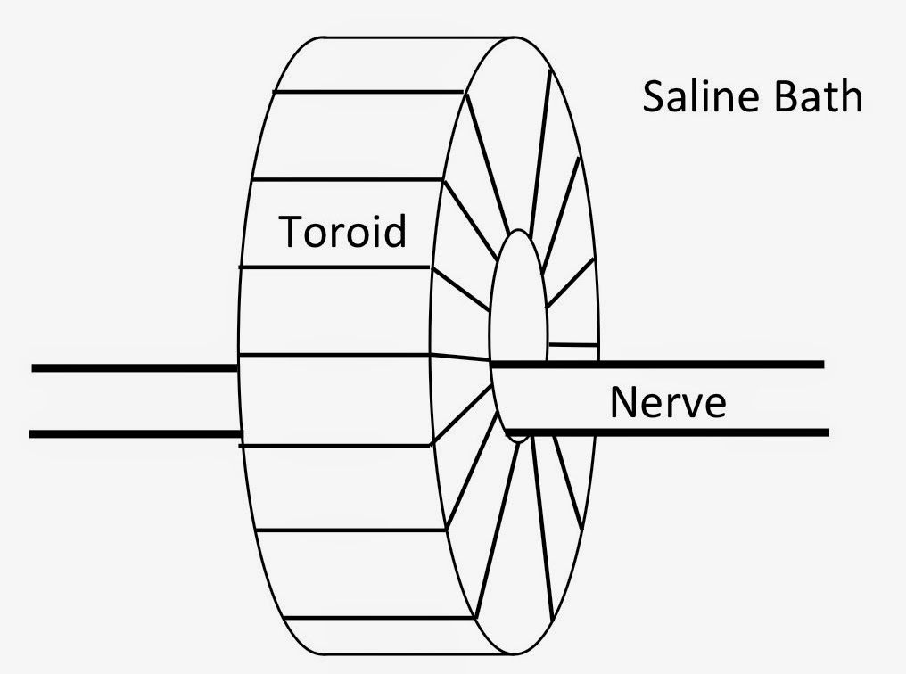
A wire-wound, ferrite-core toroid,
used to measure the magnetic field of a nerve.

To answer this question, we need to review some magnetism. Ampere’s law states that the line integral of the magnetic field around a closed path is proportional to the net current passing through a surface bounded by that path. For my experiment, that meant the magnetic signal depended on the net current passing through the toroid. The net current is the sum of the current inside the nerve axon and that fraction of the current in the saline bath that threads the toroid—the return current. In general, these currents flow in opposite directions and partially cancel. One of the difficulties I faced when interpreting my data was determining how much of the signal was from intracellular current and how much was from return current.

I struggled with this question for months. I calculated the return current with a mathematical model involving Fourier transforms and Bessel functions, but the calculation was based on many assumptions and required values for several parameters. Could I trust it? I wanted a simpler way to find the return current.

Then along came the bubble, plugging the toroid like Pooh stuck in Rabbit’s front door. The bubble blocked the return current, so the magnetic signal arose from only the intracellular current. I recorded the magnetic signal with the bubble, and then—as gently as possible—I removed the bubble and recorded the signal again. This was not easy, because surface tension makes a small bubble in water sticky, so it stuck to the toroid as if glued in place. But I eventually got rid of it without stabbing the nerve and ending the experiment.

To my delight, the magnetic field with the bubble was much larger than when it was absent. The problem of estimating the return current was solved; it’s the difference of the signal with and without the bubble. I reported this result in one of my first publications (Roth, B. J., J. K. Woosley and J. P. Wikswo, Jr., 1985, “An Experimental and Theoretical Analysis of the Magnetic Field of a Single Axon,” In: Biomagnetism: Applications and Theory, Weinberg, Stroink and Katila, Eds., Pergamon Press, New York, pp. 78–82.).

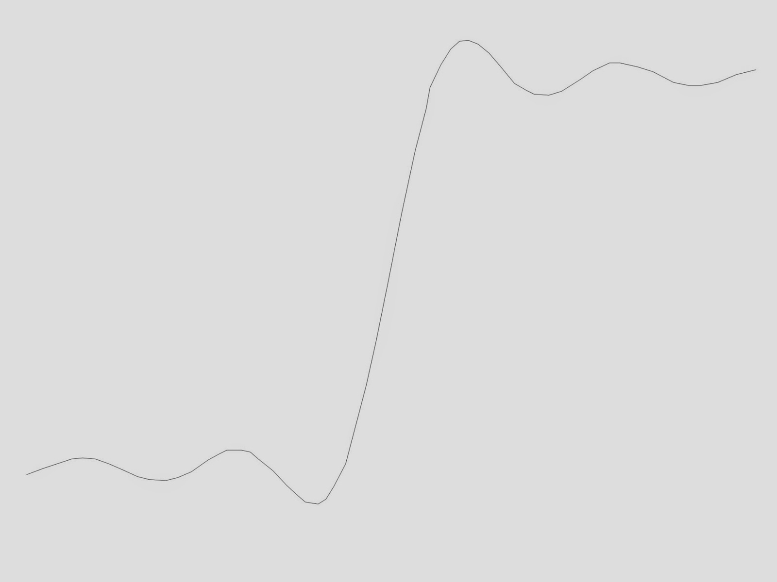
When taking data from a crayfish nerve, the toroid and axon were lifted out of the bath for a short time. […] When again placed in the bath an air bubble was trapped in the center of the toroid, filling the space between the axon and the toroid inner surface. […] Taking advantage of this fortunate occurrence, data were taken with and without the bubble present. […] The magnetic field with the bubble present […] is narrower and larger than the field with the toroid filled with saline.

The magnetic field of a nerve axon
with and without a bubble trapped
between the nerve and toroid.

On the day of the bubble experiment I was lucky. I didn’t plan the experiment. I wasn’t wise enough or thoughtful enough to realize in advance that a bubble was the ideal way to eliminate the return current. But when I looked through the dissecting microscope and saw the bubble stuck there, I was bright enough to appreciate my opportunity. “Chance favors the prepared mind.”

I have a habit of turning all my stories into homework problems. You will find the bubble story in the 4th edition of Intermediate Physics for Medicine and Biology, Problem 39 of Chapter 8. Focus on part (b).

Problem 39 A coil on a magnetic toroid as in Problem 38 is being used to measure the magnetic field of a nerve axon.

(a) If the axon is suspended in air, with only a thin layer of extracellular fluid clinging to its surface, use Ampere’s law to determine the magnetic field, B, recorded by the toroid.

(b) If the axon is immersed in a large conductor such as a saline bath, B is proportional to the sum of the intracellular current plus that fraction of the extracellular current that passes through the toroid (see Problem 13). Suppose that during an experiment an air bubble is trapped between the axon and the inner radius of the toroid? How is the magnetic signal affected by the bubble? See Roth et al. (1985).