|
| Union Station. |
I posted the last two entries in this blog while on a trip to
Kansas City to visit my parents. I didn’t grow up in the Kansas City area, but I did graduate from
Shawnee Mission South High School in
Overland Park Kansas, and I was a physics major at the
University of Kansas in
Lawrence. My dad is a native of Kansas City Missouri, while my mom moved to Kansas City Kansas when young and attended
Wyandotte High School.
 |
Kauffman Center
for the Performing Arts. |
We had a great visit, including a ride on Kansas City’s new
streetcar, which travels a route along
Main Street from
Union Station, past the
Power and Light District, within a few blocks of the
Kauffman Center, to the
River Market. We also had a great pork sandwich at
Pigwich in the East Bottoms. Kansas City is booming.
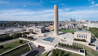 |
| Liberty Memorial. |
Is there any connection between Kansas City and medical physics? Yes, there is.
Rockhurst University, a liberal arts college located a mile west of where my dad grew up on Swope Parkway, offers an undergraduate program in the physics of medicine, which is similar to the medical physics major we offer at
Oakland University. I thought the readers of
Intermediate Physics for Medicine and Biology might like to see how another school other than Oakland structures its undergraduate medical physics curriculum.
From their Physics of Medicine
website:
POM Program Overview:
To suit your interests and career goals the POM Program has three program choices:
- Medical Physics Major - Major Track designed for students wishing to enter graduate school in Medical Physics
- Physics of Medicine (POM) Pre-Professional Major - Major Track designed for students wishing to enter a Medical/Healthcare Graduate Program
- Physics of Medicine (POM) Minor— Minor designed to complement pre-healthcare or pre-medicine program
Advantages to students of the POM Program are:
- Deeper understanding of physics principles and their applicability to a medical or health field career.
- Stronger post-graduate application to competitive health field programs.
- Undergraduate research opportunities – potential for capstone area or future graduate work.
- Value to students of interdisciplinary study, allowing them to tie together coursework in science/math with professional goals.
All Physics of Medicine Coursework is designed to complement the Scientific Foundations for Future Physicians Report, Report of the AAMC-HHMI Committee (2009).
Some courses specific to the program are:
PH 3200 Physics of the Body I:
This course expands on the physics principles developed in introductory physics courses through an in-depth study of mechanics, fluids and thermodynamics as they are applied to the human body. Areas of study include the following: biomechanics (torque, force, motion and lever systems of the body; application of vector analysis of human movement to video), thermodynamics and heat transfer (food intake and mechanical efficiency) and the pulmonary system (pressure, volume and compliance relationships). Guest speakers from the medical community will be invited.
[This course appears to cover the material in Chapters 1-3 in IPMB]
PH 3210 Physics of the Body II: This course is a continuation of Physics of the Body I with a concentration on the cardiovascular system, electricity and wave motion. Areas of study include the following: cardiovascular system (heart as a force pump, blood flow and pressure), electricity in the body (action potentials, resistance-capacitance circuit of nerve impulse propagation, EEG, EKG, EMG), and sound (hearing, voice production, sound transfer and impedance, ultrasound – transmission and reflection). In addition, students complete a guided, in-depth, individual investigation on a topic pertinent to Physics of the Body. Guest speakers from the medical community will be invited.
[Approximately Chapters 6, 7, and 13 in IPMB. PH 3200 and 3210 together are similar to Oakland University’s PHY 325, Biological Physics]
PH 3240 Physics of Medical Imaging:
This course focuses on an introduction to areas of modern physics required for an understanding of contemporary medical diagnostic and treatment procedures. Topics include a focus on the physics underlying modern medical imaging instruments: the EM Spectrum, X-Ray, CT, Gamma Camera, SPECT, PET, MRI and hybrid instrumentation. In this course, students learn about the physics involved in how these diagnostic and therapeutic instruments work as well as the numerous physics and patient factors that contribute to the choice of instrument for diagnosis. There will be field trips to local hospitals and medical imaging facilities and invited guest speakers.
[Chapters 15-18 in IPMB; similar to OU’s PHY 326, Medical Physics]
PH 4400 Optics:
This course covers both the geometric and physical properties of optical principles including optics of the eye, lasers, fiber optics, and use of endoscopy in medicine. Students will complete a final optics research project in which they relate content learned to an area of optics research.
[Chapter 14 in IPMB. We have no comparable course at OU. We offer a standard optics class, but with no biomedical emphasis. This class intrigues me.]
PH 4900 Statistics for the Health Sciences:
This course introduces the basic principles and methods of health statistics. Emphasis is on fundamental concepts and techniques of descriptive and inferential statistics with applications in health care, medicine and public health. Core content includes research design, statistical reasoning and methods. Emphasis will be on basic descriptive and inferential methods and practical applications. Data analysis tools will include descriptive statistics and graphing, confidence intervals, basic rules of probability, hypothesis testing for means and proportions, and regression analysis. Students will use specialized statistical software to conduct data analysis of health related data sets.
[Nothing exactly like this in IPMB. At OU, we require all medical physics majors to take a statistics class, taught by the Department of Mathematics and Statistics.]
PH 4900 Research in Physics of Medicine:
Independent student research on coursework from Physics of Medicine Program. Students will choose topic from Physics of Medicine Program coursework to investigate further and prepare for presentation submission. This course will serve as a capstone course for Medical Physics and Physics of Medicine Pre-Professional Majors.
[I am a big supporter of undergraduate research. At OU, medical physics majors can satisfy their capstone requirement by either research or our seminar class.]
MT 3260 Mathematical Modeling in Medicine:
Students will build mathematical models and use these models to answer questions in various areas of medicine. Topics may include: Epidemic modeling, genetics, drug treatment, bacterial population modeling, and neural systems/networks.
[IPMB is focused on mathematical modeling. I teach PHY 325 and 326 as workshops on mathematical modeling in biology and medicine.]
The Rockhurst
physics of medicine minor looks like an idea I am tempted to steal. Their requirements are:
To complete the Physics of Medicine Minor:
Prerequisites: one year of introductory/general physics and Calculus I (complete in first two years)
Upper Division Courses: complete 4 upper-division POM courses (12 hrs.total)
Required:
- PH 3200: Physics of the Body I (3 Hours, Offered Fall Semester Odd years)
- PH 3210: Physics of the Body II (3 Hours, Offered Spring Semester even years)
Choose 2 from the following:
- PH 3240: Physics of Medical Imaging (3 Hours, Offered Spring Semester Odd Years)
- PH 4400: Optics (3 hours, Offered Fall Semester Even Years)
- MT 3260: Mathematical Modeling in Medicine (3 Hours, Offered Fall Semester Even years)
- PH 4900: Statistics for the Health Sciences (3 Hours, Offered Spring semesters)
An OU version might be Biological Physics (PHY 325) and Medical Physics (PHY 326), plus their prerequisites: two semesters of introductory physics and two semesters of calculus.
 |
| The Nelson Art Gallery. |
I enjoy my trips to Kansas City because there is a lot to do and see there, from the
Nelson Art Gallery to
Crown Center to the
Liberty Memorial and the
National World War I Museum. I remember in high school attending shows at the
Starlight Theater in
Swope Park, and watching many
Kansas City Royals baseball games at
Kauffman Stadium (where I saw
George Brett play in the
World Series!). The
Truman Library is in nearby
Independence Missouri.
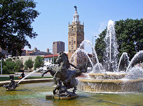 |
| The Country Club Plaza. |
I didn’t expect to find a hub of medical physics education in Kansas City, but there it is. In addition to the Rockhurst program, the
Kansas University Medical Center has a
CAMPEP-accredited clinical medical physics residency (while driving on
I-35, I could see cranes putting up a new KU Med Center building), and the
Stowers Institute, less than a mile north of Rockhurst and just east of the
Country Club Plaza, has a strong biomedical research program. As the song says,
Everything's Up To Date in Kansas City.
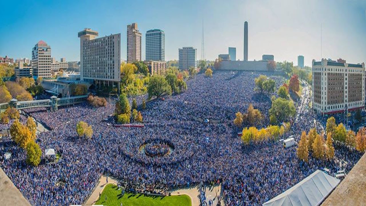 |
| Kansas City celebrating the 2015 Royals World Series Championship. |